Title
Wrapper to create plot based on provided type
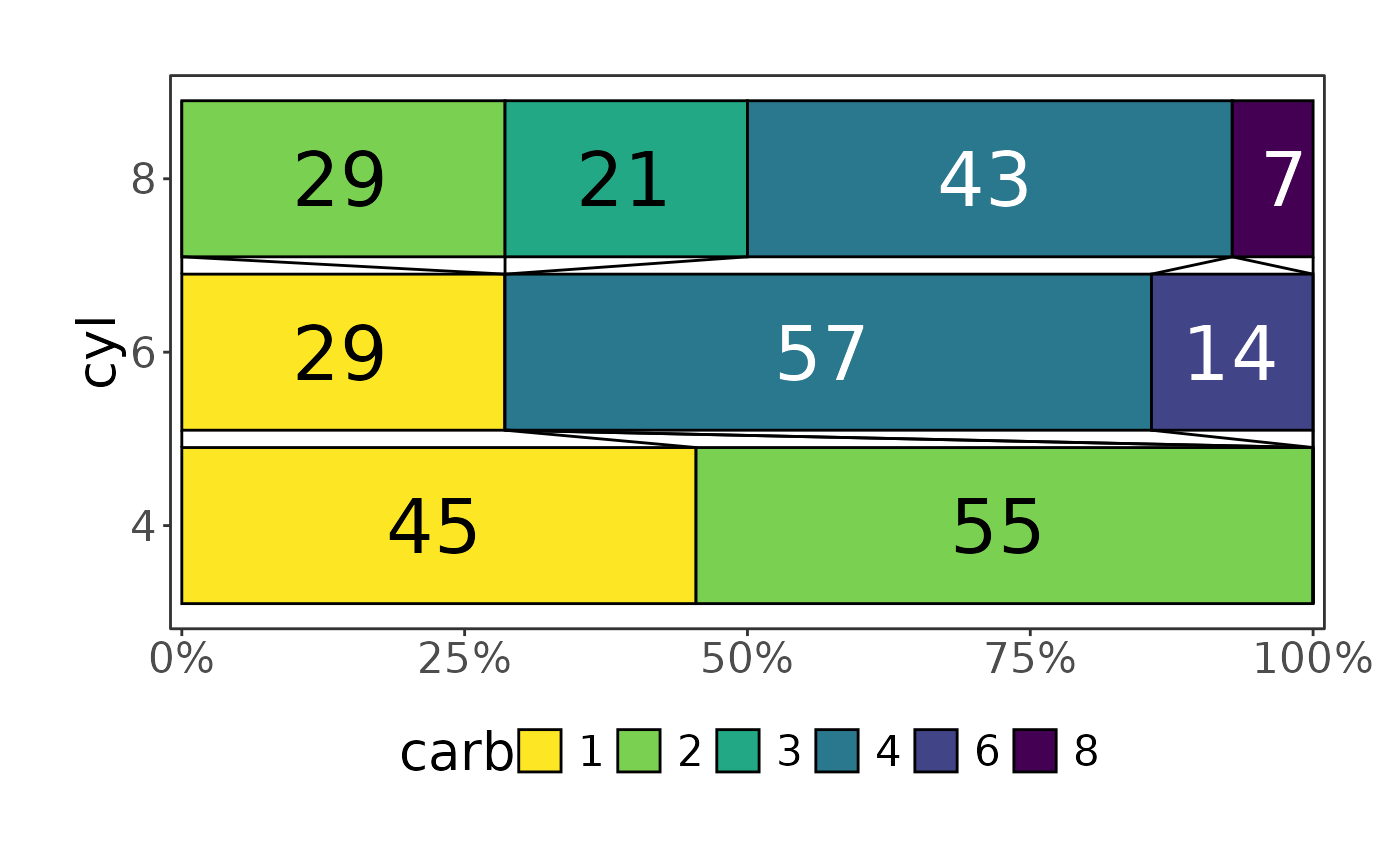
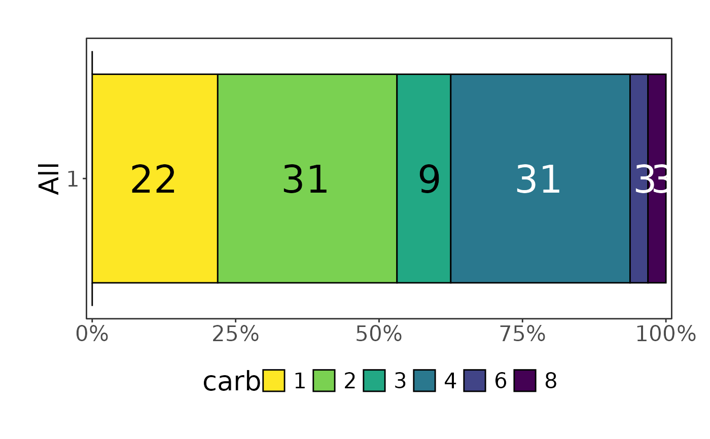
Nice horizontal stacked bars (Grotta bars)
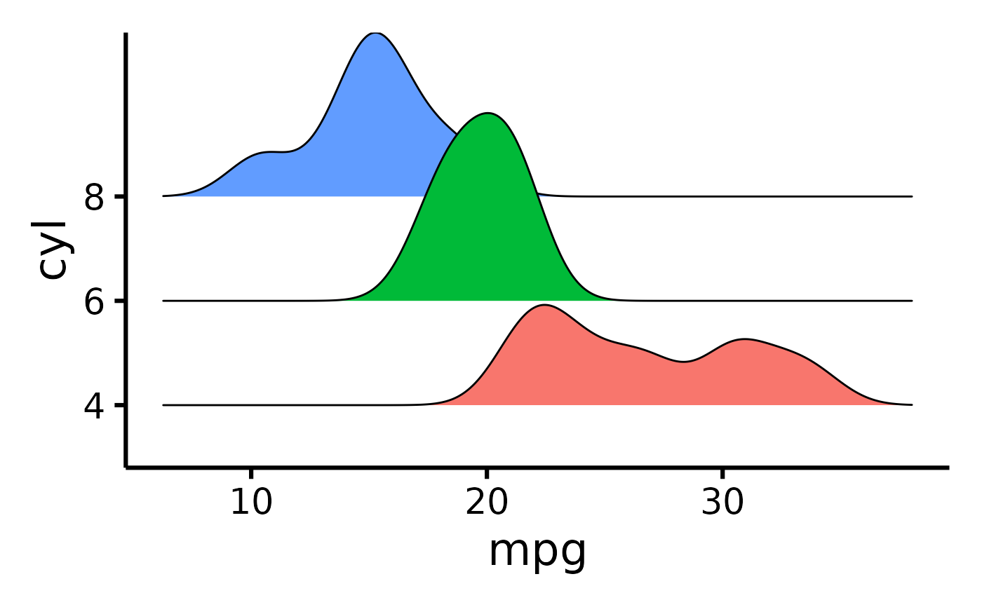
Beatiful violin plot
Beautiful violin plot
Readying data for sankey plot
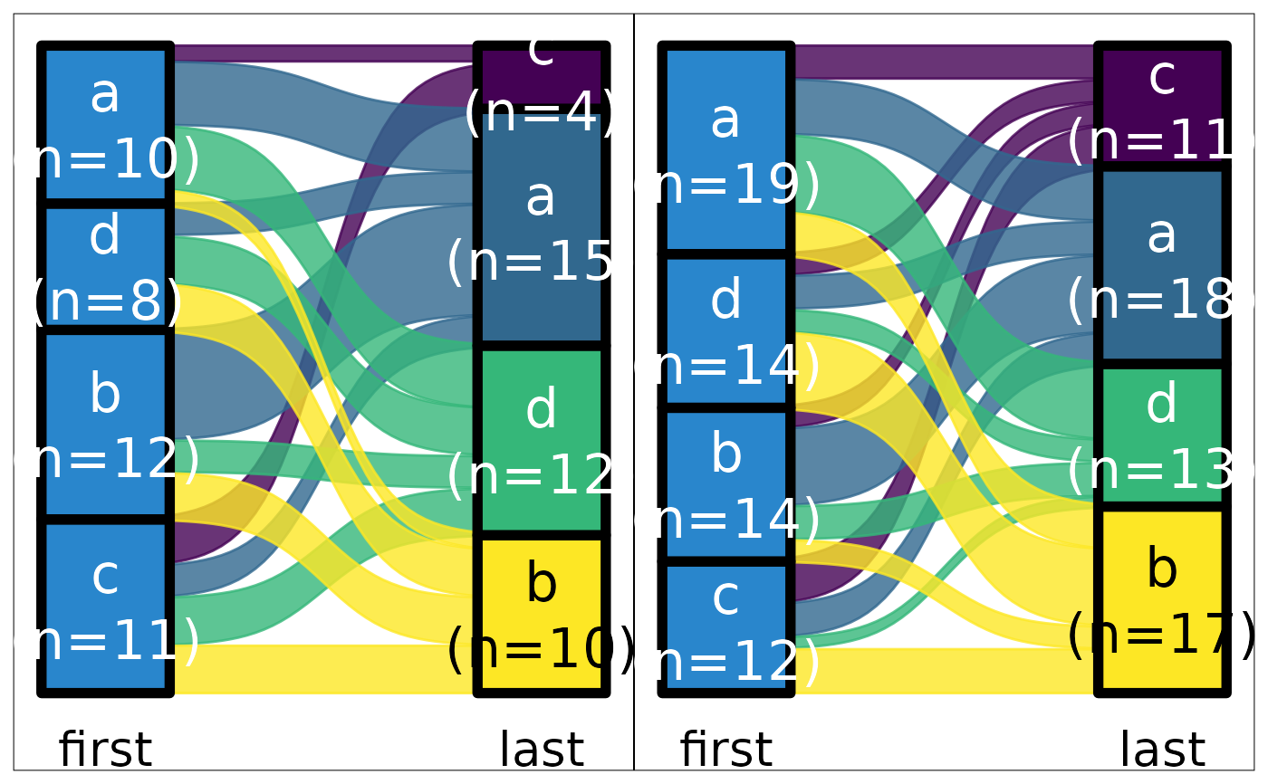
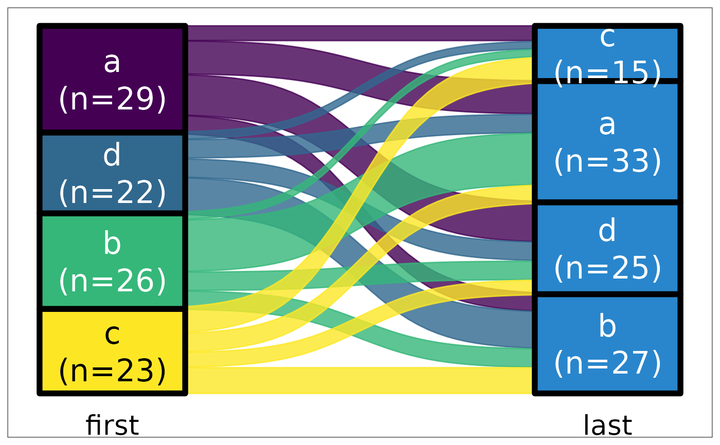
Beautiful sankey plot with option to split by a tertiary group
Usage
plot_ridge(data, x, y, z = NULL, ...)
create_plot(data, type, x, y, z = NULL, ...)
plot_hbars(data, x, y, z = NULL)
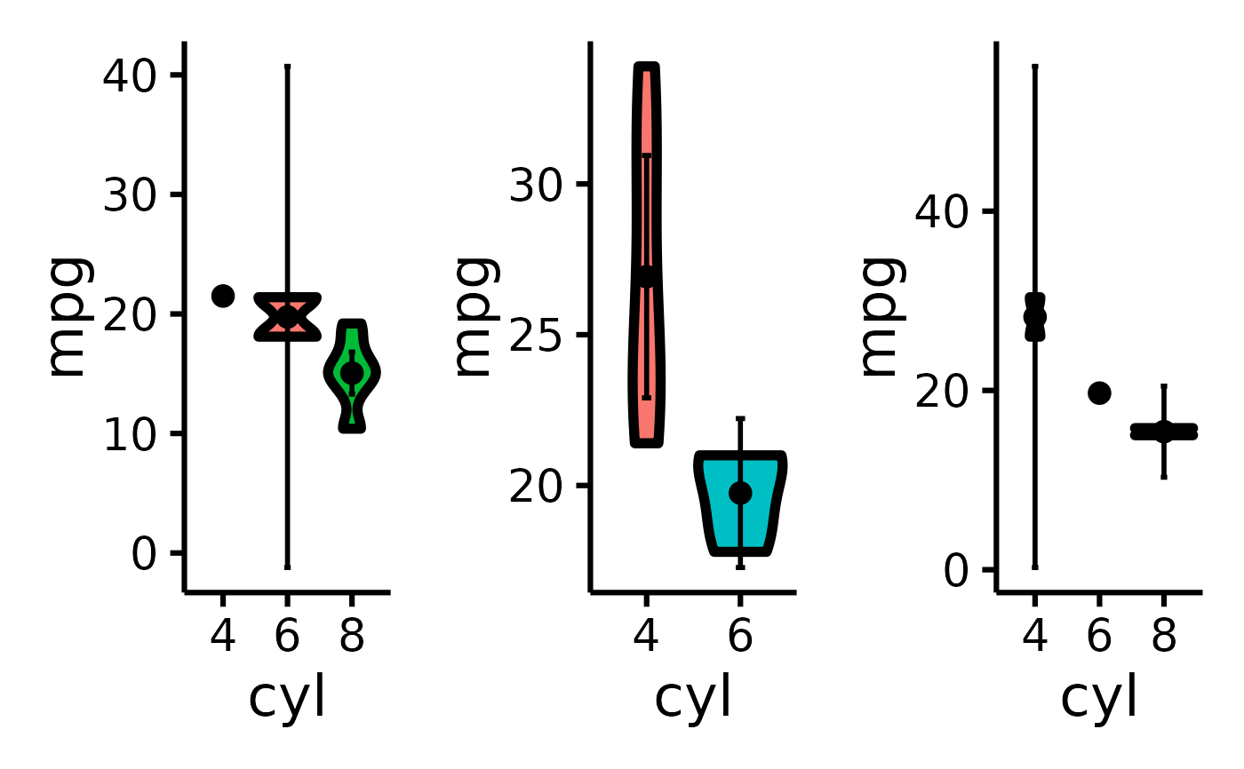
plot_violin(data, x, y, z = NULL)
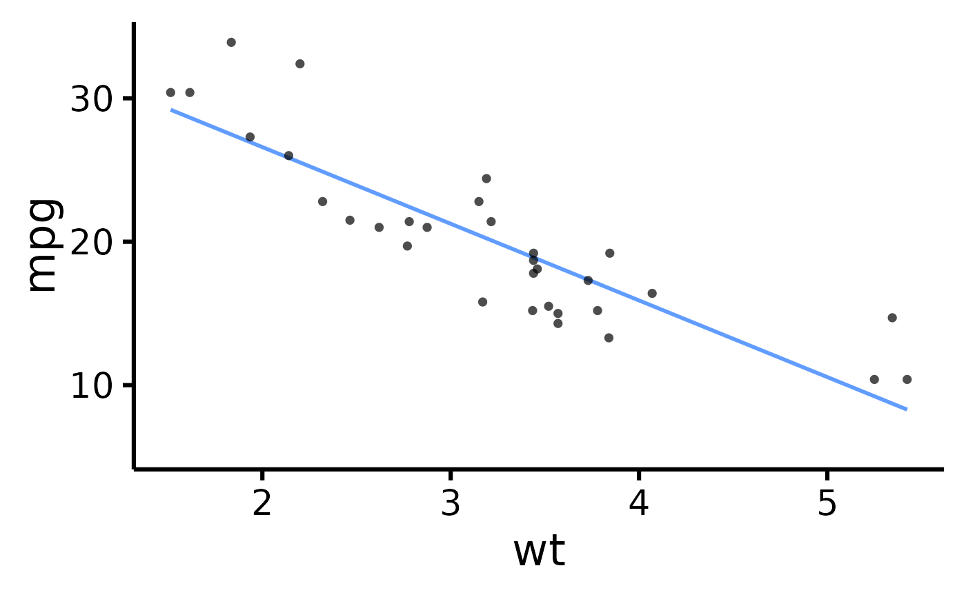
plot_scatter(data, x, y, z = NULL)
sankey_ready(data, x, y, z = NULL, numbers = "count")
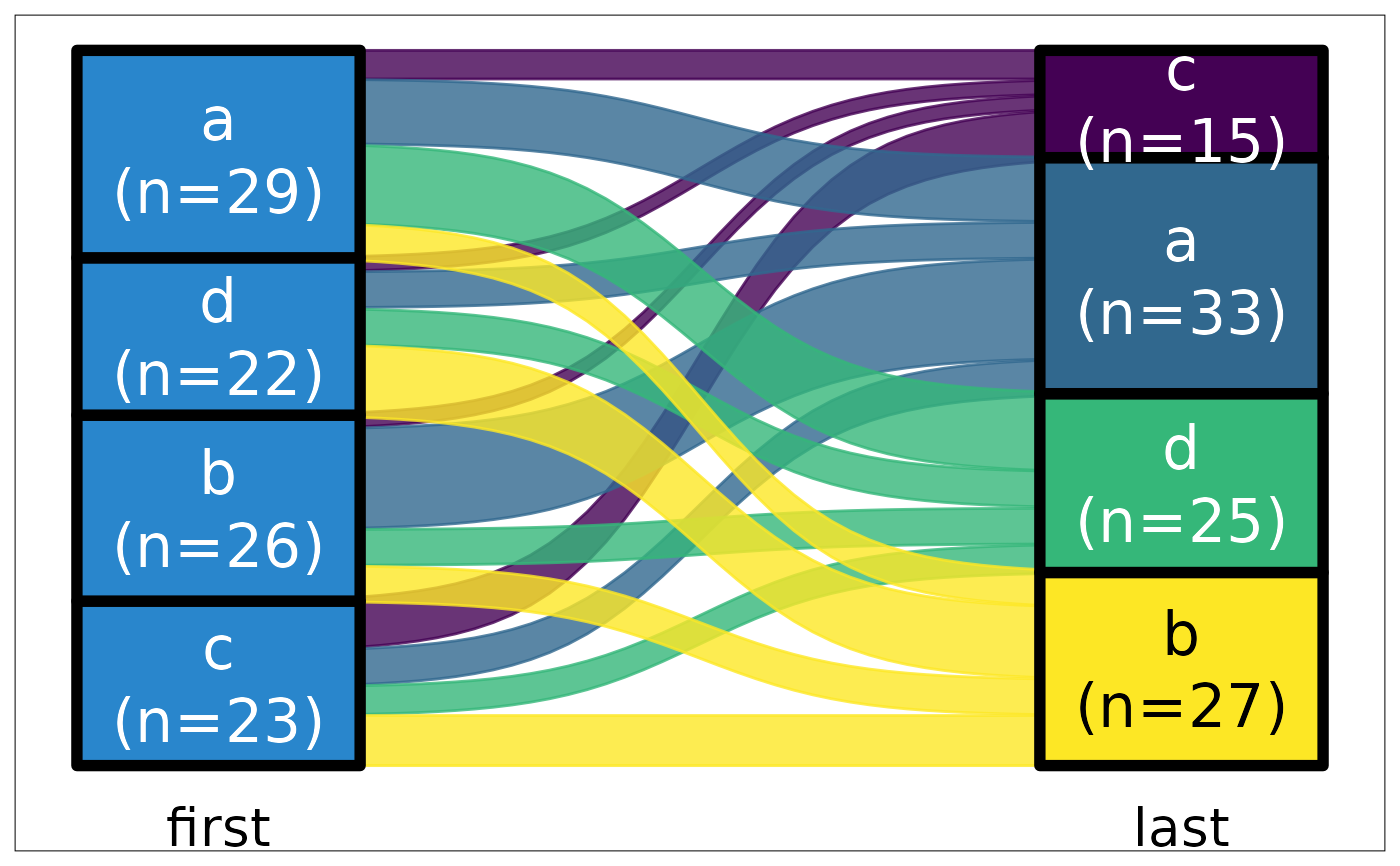
plot_sankey(data, x, y, z = NULL, color.group = "x", colors = NULL)Value
ggplot2 object
ggplot2 object
ggplot2 object
ggplot2 object
ggplot2 object
data.frame
ggplot2 object
Examples
mtcars |>
default_parsing() |>
plot_ridge(x = "mpg", y = "cyl")
#> Picking joint bandwidth of 1.38
 mtcars |> plot_ridge(x = "mpg", y = "cyl", z = "gear")
#> Picking joint bandwidth of 1.52
#> Warning: The following aesthetics were dropped during statistical transformation: y and
#> fill.
#> ℹ This can happen when ggplot fails to infer the correct grouping structure in
#> the data.
#> ℹ Did you forget to specify a `group` aesthetic or to convert a numerical
#> variable into a factor?
#> Error in ggridges::geom_density_ridges(): Problem while setting up geom.
#> ℹ Error occurred in the 1st layer.
#> Caused by error in `compute_geom_1()`:
#> ! `geom_density_ridges()` requires the following missing aesthetics: y.
create_plot(mtcars, "plot_violin", "mpg", "cyl")
#> Error in if (!z %in% names(data)) { z <- NULL}: argument is of length zero
mtcars |> plot_hbars(x = "carb", y = "cyl")
#> Scale for fill is already present.
#> Adding another scale for fill, which will replace the existing scale.
mtcars |> plot_ridge(x = "mpg", y = "cyl", z = "gear")
#> Picking joint bandwidth of 1.52
#> Warning: The following aesthetics were dropped during statistical transformation: y and
#> fill.
#> ℹ This can happen when ggplot fails to infer the correct grouping structure in
#> the data.
#> ℹ Did you forget to specify a `group` aesthetic or to convert a numerical
#> variable into a factor?
#> Error in ggridges::geom_density_ridges(): Problem while setting up geom.
#> ℹ Error occurred in the 1st layer.
#> Caused by error in `compute_geom_1()`:
#> ! `geom_density_ridges()` requires the following missing aesthetics: y.
create_plot(mtcars, "plot_violin", "mpg", "cyl")
#> Error in if (!z %in% names(data)) { z <- NULL}: argument is of length zero
mtcars |> plot_hbars(x = "carb", y = "cyl")
#> Scale for fill is already present.
#> Adding another scale for fill, which will replace the existing scale.
 mtcars |> plot_hbars(x = "carb", y = NULL)
#> Scale for fill is already present.
#> Adding another scale for fill, which will replace the existing scale.
mtcars |> plot_hbars(x = "carb", y = NULL)
#> Scale for fill is already present.
#> Adding another scale for fill, which will replace the existing scale.
 mtcars |> plot_violin(x = "mpg", y = "cyl", z = "gear")
#> Warning: There was 1 warning in `summarize()`.
#> ℹ In argument: `V1 = .fun(as.data.frame(pick(everything())), var)`.
#> ℹ In group 1: `cyl = 4`.
#> Caused by warning in `stats::qt()`:
#> ! NaNs produced
#> Warning: There was 1 warning in `summarize()`.
#> ℹ In argument: `V1 = .fun(as.data.frame(pick(everything())), var)`.
#> ℹ In group 1: `cyl = 4`.
#> Caused by warning in `stats::qt()`:
#> ! NaNs produced
#> Warning: There was 1 warning in `summarize()`.
#> ℹ In argument: `V1 = .fun(as.data.frame(pick(everything())), var)`.
#> ℹ In group 2: `cyl = 6`.
#> Caused by warning in `stats::qt()`:
#> ! NaNs produced
#> Warning: There was 1 warning in `summarize()`.
#> ℹ In argument: `V1 = .fun(as.data.frame(pick(everything())), var)`.
#> ℹ In group 2: `cyl = 6`.
#> Caused by warning in `stats::qt()`:
#> ! NaNs produced
#> Warning: Groups with fewer than two datapoints have been dropped.
#> ℹ Set `drop = FALSE` to consider such groups for position adjustment purposes.
#> Warning: Groups with fewer than two datapoints have been dropped.
#> ℹ Set `drop = FALSE` to consider such groups for position adjustment purposes.
mtcars |> plot_violin(x = "mpg", y = "cyl", z = "gear")
#> Warning: There was 1 warning in `summarize()`.
#> ℹ In argument: `V1 = .fun(as.data.frame(pick(everything())), var)`.
#> ℹ In group 1: `cyl = 4`.
#> Caused by warning in `stats::qt()`:
#> ! NaNs produced
#> Warning: There was 1 warning in `summarize()`.
#> ℹ In argument: `V1 = .fun(as.data.frame(pick(everything())), var)`.
#> ℹ In group 1: `cyl = 4`.
#> Caused by warning in `stats::qt()`:
#> ! NaNs produced
#> Warning: There was 1 warning in `summarize()`.
#> ℹ In argument: `V1 = .fun(as.data.frame(pick(everything())), var)`.
#> ℹ In group 2: `cyl = 6`.
#> Caused by warning in `stats::qt()`:
#> ! NaNs produced
#> Warning: There was 1 warning in `summarize()`.
#> ℹ In argument: `V1 = .fun(as.data.frame(pick(everything())), var)`.
#> ℹ In group 2: `cyl = 6`.
#> Caused by warning in `stats::qt()`:
#> ! NaNs produced
#> Warning: Groups with fewer than two datapoints have been dropped.
#> ℹ Set `drop = FALSE` to consider such groups for position adjustment purposes.
#> Warning: Groups with fewer than two datapoints have been dropped.
#> ℹ Set `drop = FALSE` to consider such groups for position adjustment purposes.
 mtcars |> plot_scatter(x = "mpg", y = "wt")
 ds <- data.frame(g = sample(LETTERS[1:2], 100, TRUE), first = REDCapCAST::as_factor(sample(letters[1:4], 100, TRUE)), last = sample(c(letters[1:4], NA), 100, TRUE, prob = c(rep(.23, 4), .08)))
ds |> sankey_ready("first", "last")
#> # A tibble: 19 × 7
#> first last n gx.sum gy.sum lx ly
#> <fct> <chr> <int> <int> <int> <fct> <fct>
#> 1 c a 7 28 32 "c\n(n=28)" "a\n(n=32)"
#> 2 c b 6 28 26 "c\n(n=28)" "b\n(n=26)"
#> 3 c c 5 28 15 "c\n(n=28)" "c\n(n=15)"
#> 4 c d 6 28 17 "c\n(n=28)" "d\n(n=17)"
#> 5 c NA 4 28 10 "c\n(n=28)" "NA\n(n=10)"
#> 6 a a 9 24 32 "a\n(n=24)" "a\n(n=32)"
#> 7 a b 6 24 26 "a\n(n=24)" "b\n(n=26)"
#> 8 a c 6 24 15 "a\n(n=24)" "c\n(n=15)"
#> 9 a d 1 24 17 "a\n(n=24)" "d\n(n=17)"
#> 10 a NA 2 24 10 "a\n(n=24)" "NA\n(n=10)"
#> 11 b a 8 20 32 "b\n(n=20)" "a\n(n=32)"
#> 12 b b 5 20 26 "b\n(n=20)" "b\n(n=26)"
#> 13 b c 4 20 15 "b\n(n=20)" "c\n(n=15)"
#> 14 b d 2 20 17 "b\n(n=20)" "d\n(n=17)"
#> 15 b NA 1 20 10 "b\n(n=20)" "NA\n(n=10)"
#> 16 d a 8 28 32 "d\n(n=28)" "a\n(n=32)"
#> 17 d b 9 28 26 "d\n(n=28)" "b\n(n=26)"
#> 18 d d 8 28 17 "d\n(n=28)" "d\n(n=17)"
#> 19 d NA 3 28 10 "d\n(n=28)" "NA\n(n=10)"
ds |> sankey_ready("first", "last", numbers = "percentage")
#> # A tibble: 19 × 7
#> first last n gx.sum gy.sum lx ly
#> <fct> <chr> <int> <int> <int> <fct> <fct>
#> 1 c a 7 28 32 "c\n(28%)" "a\n(32%)"
#> 2 c b 6 28 26 "c\n(28%)" "b\n(26%)"
#> 3 c c 5 28 15 "c\n(28%)" "c\n(15%)"
#> 4 c d 6 28 17 "c\n(28%)" "d\n(17%)"
#> 5 c NA 4 28 10 "c\n(28%)" "NA\n(10%)"
#> 6 a a 9 24 32 "a\n(24%)" "a\n(32%)"
#> 7 a b 6 24 26 "a\n(24%)" "b\n(26%)"
#> 8 a c 6 24 15 "a\n(24%)" "c\n(15%)"
#> 9 a d 1 24 17 "a\n(24%)" "d\n(17%)"
#> 10 a NA 2 24 10 "a\n(24%)" "NA\n(10%)"
#> 11 b a 8 20 32 "b\n(20%)" "a\n(32%)"
#> 12 b b 5 20 26 "b\n(20%)" "b\n(26%)"
#> 13 b c 4 20 15 "b\n(20%)" "c\n(15%)"
#> 14 b d 2 20 17 "b\n(20%)" "d\n(17%)"
#> 15 b NA 1 20 10 "b\n(20%)" "NA\n(10%)"
#> 16 d a 8 28 32 "d\n(28%)" "a\n(32%)"
#> 17 d b 9 28 26 "d\n(28%)" "b\n(26%)"
#> 18 d d 8 28 17 "d\n(28%)" "d\n(17%)"
#> 19 d NA 3 28 10 "d\n(28%)" "NA\n(10%)"
ds <- data.frame(g = sample(LETTERS[1:2], 100, TRUE), first = REDCapCAST::as_factor(sample(letters[1:4], 100, TRUE)), last = REDCapCAST::as_factor(sample(letters[1:4], 100, TRUE)))
ds |> plot_sankey("first", "last")
#> Loading required package: ggplot2
ds <- data.frame(g = sample(LETTERS[1:2], 100, TRUE), first = REDCapCAST::as_factor(sample(letters[1:4], 100, TRUE)), last = sample(c(letters[1:4], NA), 100, TRUE, prob = c(rep(.23, 4), .08)))
ds |> sankey_ready("first", "last")
#> # A tibble: 19 × 7
#> first last n gx.sum gy.sum lx ly
#> <fct> <chr> <int> <int> <int> <fct> <fct>
#> 1 c a 7 28 32 "c\n(n=28)" "a\n(n=32)"
#> 2 c b 6 28 26 "c\n(n=28)" "b\n(n=26)"
#> 3 c c 5 28 15 "c\n(n=28)" "c\n(n=15)"
#> 4 c d 6 28 17 "c\n(n=28)" "d\n(n=17)"
#> 5 c NA 4 28 10 "c\n(n=28)" "NA\n(n=10)"
#> 6 a a 9 24 32 "a\n(n=24)" "a\n(n=32)"
#> 7 a b 6 24 26 "a\n(n=24)" "b\n(n=26)"
#> 8 a c 6 24 15 "a\n(n=24)" "c\n(n=15)"
#> 9 a d 1 24 17 "a\n(n=24)" "d\n(n=17)"
#> 10 a NA 2 24 10 "a\n(n=24)" "NA\n(n=10)"
#> 11 b a 8 20 32 "b\n(n=20)" "a\n(n=32)"
#> 12 b b 5 20 26 "b\n(n=20)" "b\n(n=26)"
#> 13 b c 4 20 15 "b\n(n=20)" "c\n(n=15)"
#> 14 b d 2 20 17 "b\n(n=20)" "d\n(n=17)"
#> 15 b NA 1 20 10 "b\n(n=20)" "NA\n(n=10)"
#> 16 d a 8 28 32 "d\n(n=28)" "a\n(n=32)"
#> 17 d b 9 28 26 "d\n(n=28)" "b\n(n=26)"
#> 18 d d 8 28 17 "d\n(n=28)" "d\n(n=17)"
#> 19 d NA 3 28 10 "d\n(n=28)" "NA\n(n=10)"
ds |> sankey_ready("first", "last", numbers = "percentage")
#> # A tibble: 19 × 7
#> first last n gx.sum gy.sum lx ly
#> <fct> <chr> <int> <int> <int> <fct> <fct>
#> 1 c a 7 28 32 "c\n(28%)" "a\n(32%)"
#> 2 c b 6 28 26 "c\n(28%)" "b\n(26%)"
#> 3 c c 5 28 15 "c\n(28%)" "c\n(15%)"
#> 4 c d 6 28 17 "c\n(28%)" "d\n(17%)"
#> 5 c NA 4 28 10 "c\n(28%)" "NA\n(10%)"
#> 6 a a 9 24 32 "a\n(24%)" "a\n(32%)"
#> 7 a b 6 24 26 "a\n(24%)" "b\n(26%)"
#> 8 a c 6 24 15 "a\n(24%)" "c\n(15%)"
#> 9 a d 1 24 17 "a\n(24%)" "d\n(17%)"
#> 10 a NA 2 24 10 "a\n(24%)" "NA\n(10%)"
#> 11 b a 8 20 32 "b\n(20%)" "a\n(32%)"
#> 12 b b 5 20 26 "b\n(20%)" "b\n(26%)"
#> 13 b c 4 20 15 "b\n(20%)" "c\n(15%)"
#> 14 b d 2 20 17 "b\n(20%)" "d\n(17%)"
#> 15 b NA 1 20 10 "b\n(20%)" "NA\n(10%)"
#> 16 d a 8 28 32 "d\n(28%)" "a\n(32%)"
#> 17 d b 9 28 26 "d\n(28%)" "b\n(26%)"
#> 18 d d 8 28 17 "d\n(28%)" "d\n(17%)"
#> 19 d NA 3 28 10 "d\n(28%)" "NA\n(10%)"
ds <- data.frame(g = sample(LETTERS[1:2], 100, TRUE), first = REDCapCAST::as_factor(sample(letters[1:4], 100, TRUE)), last = REDCapCAST::as_factor(sample(letters[1:4], 100, TRUE)))
ds |> plot_sankey("first", "last")
#> Loading required package: ggplot2
 ds |> plot_sankey("first", "last", color.group = "y")
 ds |> plot_sankey("first", "last", z = "g", color.group = "y")