Beautiful sankey plot
Usage
plot_sankey_single(
  data,
  pri,
  sec,
  color.group = c("pri", "sec"),
  colors = NULL,
  ...
)Examples
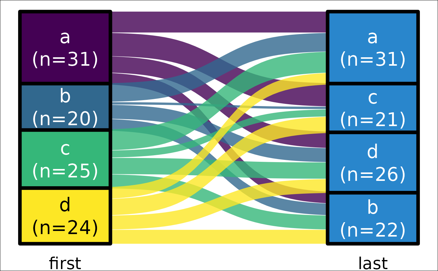
ds <- data.frame(g = sample(LETTERS[1:2], 100, TRUE), first = REDCapCAST::as_factor(sample(letters[1:4], 100, TRUE)), last = REDCapCAST::as_factor(sample(letters[1:4], 100, TRUE)))
ds |> plot_sankey_single("first", "last")
#> Warning: Some strata appear at multiple axes.
#> Warning: Some strata appear at multiple axes.
#> Warning: Some strata appear at multiple axes.
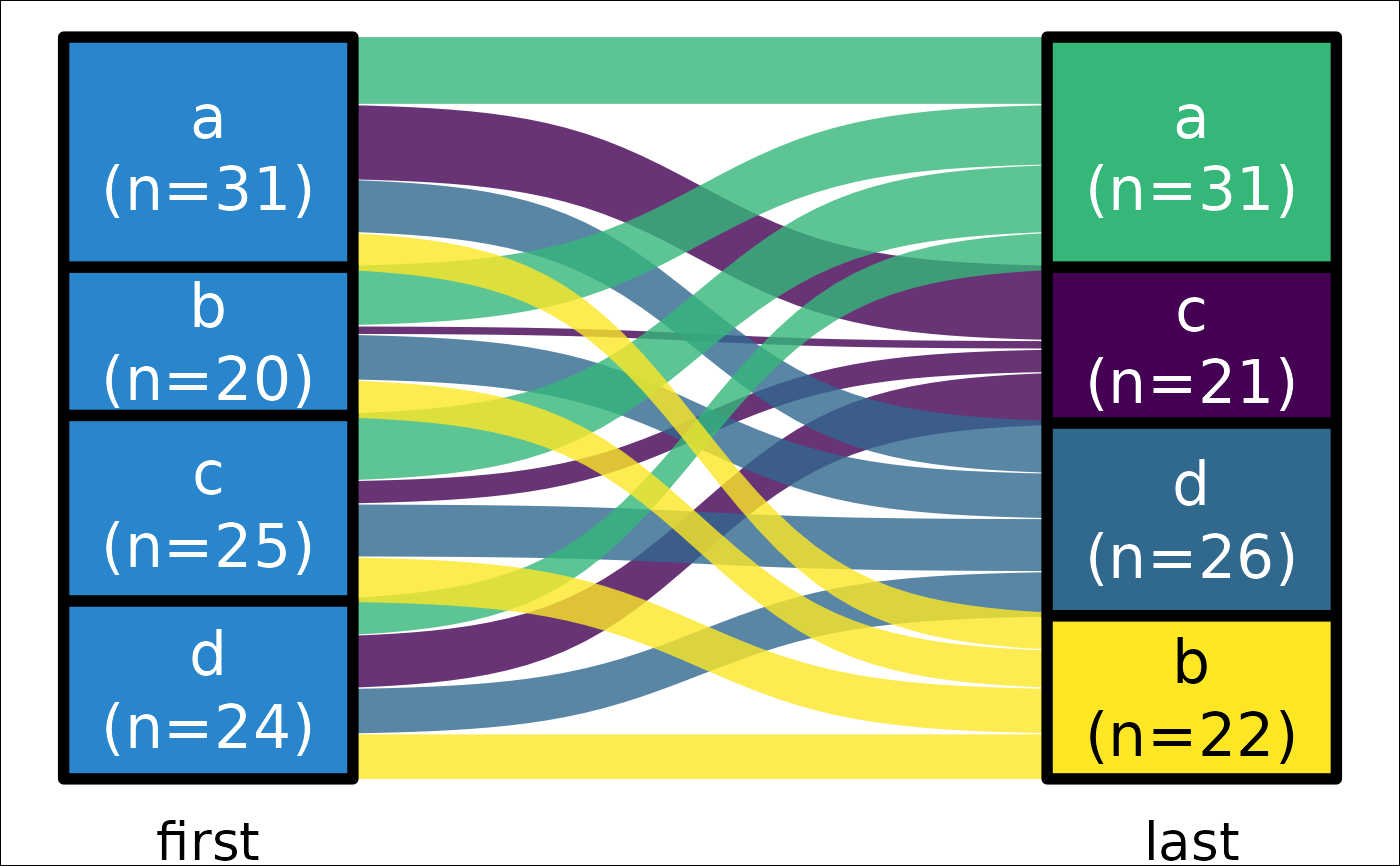
 ds |> plot_sankey_single("first", "last", color.group = "sec")
#> Warning: Some strata appear at multiple axes.
#> Warning: Some strata appear at multiple axes.
#> Warning: Some strata appear at multiple axes.
ds |> plot_sankey_single("first", "last", color.group = "sec")
#> Warning: Some strata appear at multiple axes.
#> Warning: Some strata appear at multiple axes.
#> Warning: Some strata appear at multiple axes.
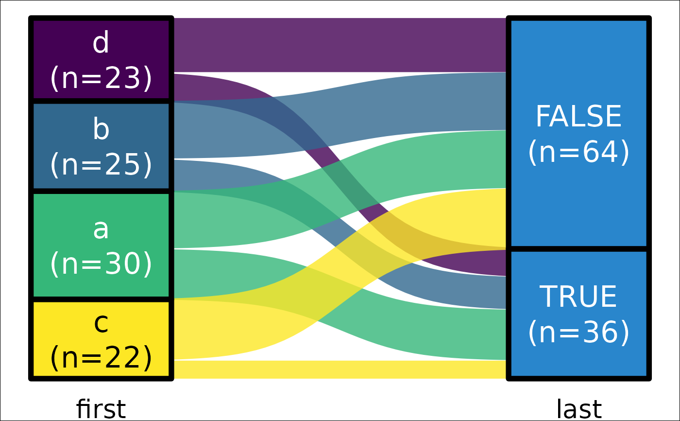
 data.frame(
g = sample(LETTERS[1:2], 100, TRUE),
first = REDCapCAST::as_factor(sample(letters[1:4], 100, TRUE)),
last = sample(c(TRUE, FALSE, FALSE), 100, TRUE)
) |>
plot_sankey_single("first", "last", color.group = "pri")
data.frame(
g = sample(LETTERS[1:2], 100, TRUE),
first = REDCapCAST::as_factor(sample(letters[1:4], 100, TRUE)),
last = sample(c(TRUE, FALSE, FALSE), 100, TRUE)
) |>
plot_sankey_single("first", "last", color.group = "pri")
 mtcars |>
default_parsing() |>
str()
#> tibble [32 × 11] (S3: tbl_df/tbl/data.frame)
#> $ mpg : num [1:32] 21 21 22.8 21.4 18.7 18.1 14.3 24.4 22.8 19.2 ...
#> $ cyl : Factor w/ 3 levels "4","6","8": 2 2 1 2 3 2 3 1 1 2 ...
#> $ disp: num [1:32] 160 160 108 258 360 ...
#> $ hp : num [1:32] 110 110 93 110 175 105 245 62 95 123 ...
#> $ drat: num [1:32] 3.9 3.9 3.85 3.08 3.15 2.76 3.21 3.69 3.92 3.92 ...
#> $ wt : num [1:32] 2.62 2.88 2.32 3.21 3.44 ...
#> $ qsec: num [1:32] 16.5 17 18.6 19.4 17 ...
#> $ vs : logi [1:32] FALSE FALSE TRUE TRUE FALSE TRUE ...
#> $ am : logi [1:32] TRUE TRUE TRUE FALSE FALSE FALSE ...
#> $ gear: Factor w/ 3 levels "3","4","5": 2 2 2 1 1 1 1 2 2 2 ...
#> $ carb: Factor w/ 6 levels "1","2","3","4",..: 4 4 1 1 2 1 4 2 2 4 ...
plot_sankey_single("cyl", "vs", color.group = "pri")
#> Error in plot_sankey_single("cyl", "vs", color.group = "pri"): argument "sec" is missing, with no default
mtcars |>
default_parsing() |>
str()
#> tibble [32 × 11] (S3: tbl_df/tbl/data.frame)
#> $ mpg : num [1:32] 21 21 22.8 21.4 18.7 18.1 14.3 24.4 22.8 19.2 ...
#> $ cyl : Factor w/ 3 levels "4","6","8": 2 2 1 2 3 2 3 1 1 2 ...
#> $ disp: num [1:32] 160 160 108 258 360 ...
#> $ hp : num [1:32] 110 110 93 110 175 105 245 62 95 123 ...
#> $ drat: num [1:32] 3.9 3.9 3.85 3.08 3.15 2.76 3.21 3.69 3.92 3.92 ...
#> $ wt : num [1:32] 2.62 2.88 2.32 3.21 3.44 ...
#> $ qsec: num [1:32] 16.5 17 18.6 19.4 17 ...
#> $ vs : logi [1:32] FALSE FALSE TRUE TRUE FALSE TRUE ...
#> $ am : logi [1:32] TRUE TRUE TRUE FALSE FALSE FALSE ...
#> $ gear: Factor w/ 3 levels "3","4","5": 2 2 2 1 1 1 1 2 2 2 ...
#> $ carb: Factor w/ 6 levels "1","2","3","4",..: 4 4 1 1 2 1 4 2 2 4 ...
plot_sankey_single("cyl", "vs", color.group = "pri")
#> Error in plot_sankey_single("cyl", "vs", color.group = "pri"): argument "sec" is missing, with no default